Jupyter
Project Jupyter is a collection of open-source software, open-standards, and services for interactive computing across a variety of programming languages. We use Jupyter with Python as a core tool for analysis of model results and ocean observations, and communication of those analyses within the MOAD group, and with collaborators.
Jupyter Notebooks are the core feature of Jupyter. Notebooks contain live Python code, equations, visualizations, and narrative text. They are an excellent tool for data exploration and analysis, teaching, communication, and early-stage code development.
Jupyter is a server-client system, even when you are running it on your own laptop. The server part runs in a terminal window and is called the kernel. It’s the part that runs Python. The client part runs in your web browser. It’s the part where you type in code, narrative text, LaTeX equations, etc. and where you see the code results and visualization images.
Jupyter provides more than one user interface, among them:
The original jupyter notebook interface opens a file navigator in one tab of your browser. Clicking on a notebooks in that navigator tab causes it to open in another browser tab. You can open as many notebook tabs as you want - at least until your computer runs out of memory!
The jupyter lab is the newer “next generation” interface that puts everything in one browser tab with multiple panes that you can move around and re-size. In addition to notebooks,
labalso provides a text editor, code consoles that are synced with notebooks, and terminal panes that give access to your system shell, just like your terminal program does.VS Code also provides the ability to edit and run Jupyter notebooks directly in the VS Code interface.
VS Code is probably the easiest way to work with Jupyter notebooks
if you are already using VS Code for other coding tasks.
However,
if you prefer the browser-based interfaces,
you should use the lab interface because that is the part of Jupyter that is being most actively developed,
and where new features are most likely to appear.
Notebooks aren’t the only way to use Python though! Code that is frequently used, that is hundreds of lines long, or that takes a significant amount of time to run is often best moved from notebooks into Python modules and packages. Doing so makes the code more maintainable, testable, and more efficient to run, but at the expense of separating the code from equations, visualizations, and narrative text. Those important things have to find a home in documentation that accompanies the code modules.
Running Jupyter Locally
Assuming that you have Installed Miniforge so that
you are using conda to create and manage your Python environments,
you can install Jupyter by adding the jupyterlab package to your environment description YAML file.
For example,
the notebooks/environment.yaml file in your analysis repo includes jupyterlab.
Using VS Code
Ensure that you have the Python extension installed in VS Code. See the Recommended Extensions section for instructions.
Open the notebook file you want to work on in VS Code, either by using the File > Open File… menu, or by opening the analysis repo folder in VS Code and using the Explorer sidebar to navigate to and open the notebook file.
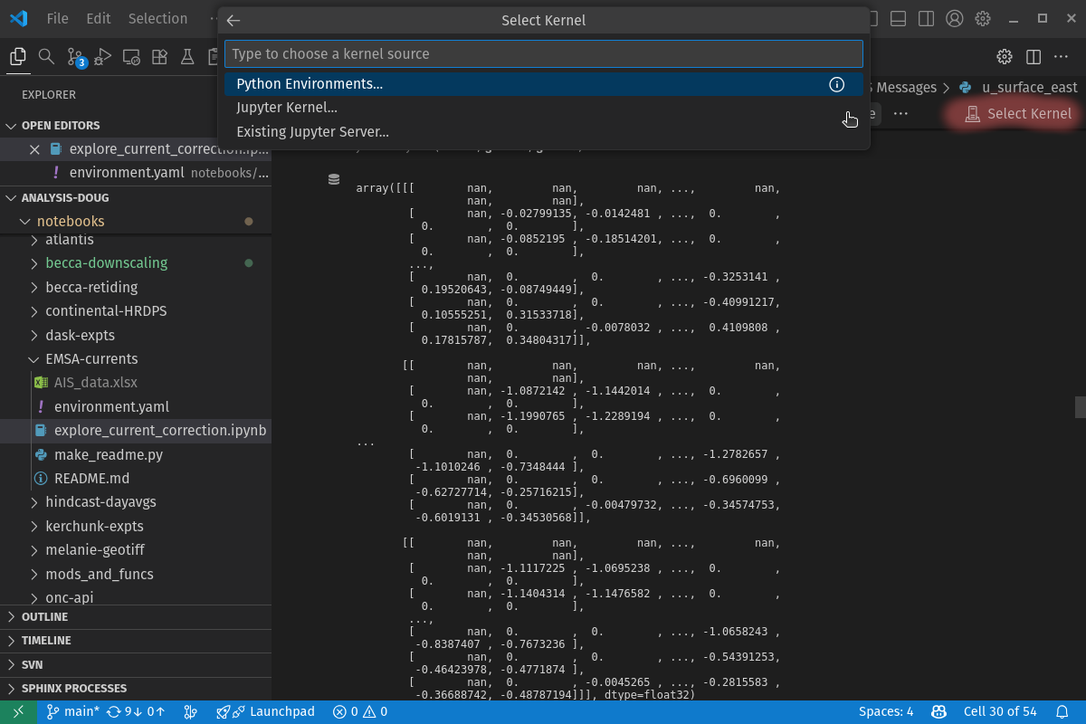
If the Python environment that you want to use for the notebook is not already selected, use the Select Kernel button in the upper right corner of the notebook editor pane (highlighted in the figure below) to choose the correct environment. You should see a list of available Python environments including the one you created for your analysis repo. Select that environment to use it as the kernel for the notebook.
The “Jupyter Notebook quick start” section of the Microsoft Python extension page has more details and links about using Jupyter notebooks in VS Code.
Using a Terminal Window
In a terminal window, go to the directory that you want to be at the top level of Jupyter’s file navigation, and start the Jupyter server. For example, if you are working in your analysis repo, the commands would be like:
$ conda activate analysis-doug
(analysis-doug)$ cd analysis-doug/
(analysis-doug)$ jupyter lab
The terminal window that you typed those commands into is now running the server part of Jupyter. You have to keep it open until you are finished with Jupyter and want to shut it down.
The client part of Jupyter should have opened in a new browser tab. If not, follow the instructions in the terminal window that say something like:
For the older notebook interface,
the instructions are much the same,
but the command to start the server is jupyter notebook.
When you are finished using Jupyter, save your notebook(s) via the menu in the browser tab, close the tab, and use Ctrl-C in the terminal window to shut down the Jupyter server.
Don’t forget to commit your work in git and push your changes to GitHub!
Running Jupyter Remotely
Running Jupyter Locally is fine if your laptop has enough compute power for the code you are trying to run,
and if you have the data or model results files you want to work on stored on your drive.
However,
it is often better to “take the compute to the data” rather than download large data files to your laptop,
and rely on its CPU cores for calculations.
Remote machines like the MOAD workstations,
our development server salish,
and the compute nodes on the Alliance nibi cluster
have more and faster CPU cores than most laptops,
and access to far larger storage.
Fortunately, the server-client structure of Jupyter makes it relatively easy to use the CPU cores and storage of a remote system with the user interface in the browser on your laptop. We do that by running the server part on a remote system, and using ssh to create a secure access “tunnel” between the server and our laptop to allow the client part running in our local browser to connect to the remote server part. Again, the easiest way to do that is to use VS Code with its Remote SSH Extension.
If you decided to use the browser-based Jupyter interfaces rather than VS Code, the jupyter lab interface provides some useful tools on the remote system that are similar to what you get with VS Code:
You can open terminal panes in the
labinterface to give you a terminal session on the remote machine for things like file system tasks: copying or moving files, managing permissions, etc., for git version control tasks: pulls, commits, and pushes, or anything else you need to do in a command-line interface.You can open editor panes in the
labinterface to work on files stored on the remote system. Doing that avoids the need to copy files back and forth between your laptop and the remote system, or deal with network lag when you try to use a full-screen editor in a remote desktop session. You can use the Settings > Text Editor Key Map menu inlabto set the editor keyboard mapping to your choice of vim, emacs, or Sublime Text.
Running Jupyter Remotely on salish or a MOAD Workstation
This section assumes that you have Installed Miniforge
in your $HOME directory on a MOAD workstation,
or that you are working in conda environment that includes the jupyterlab package on a MOAD workstation.
Note
You don’t need to Install Miniforge or jupyterlab
explicitly on salish if you have already installed it on a MOAD workstation because salish uses the same $HOME file system as all of the MOAD workstations.
It is also assumed that you have followed the instructions in the Set Up ssh Configuration section to set up host aliases for salish and any other workstations you want to run the jupyter lab server on.
You can use the technique in this section to run the jupyter lab server on any of the MOAD workstations by replacing salish with the workstation name.
salish has the advantages of having lots of compute power
(16 3.2 MHz cores running 2 threads each,
and 256 Gb of memory)
and of being close physically and in network terms to our large storage arrays /data/,
/results/,
/results2/,
/opp/,
and /ocean/.
That said,
the MOAD workstations have ample compute power and are nearly as fast access to the storage arrays,
so they are well up to the task of running the jupyter lab for analysis work.
Using VS Code
Ensure that you have the Remote SSH extension installed in VS Code. See the Remote - SSH Extension Notes section for details.
Use the Remote - SSH extension to open a VS Code window connected to
salishor a MOAD workstation.Ensure that you have the Python extension installed for VS Code on the remote machine.
If you haven’t already done so, clone the repository containing the notebook(s) you want to use on the remote machine, and create the conda environment for it.
Open the notebook file you want to work on in VS Code, either by using the File > Open File… menu, or by opening the analysis repo folder in VS Code and using the Explorer sidebar to navigate to and open the notebook file.
If the Python environment that you want to use for the notebook is not already selected, use the Select Kernel button in the upper right corner of the notebook editor pane (highlighted in the figure below) to choose the correct environment. You should see a list of available Python environments including the one you created for your analysis repo. Select that environment to use it as the kernel for the notebook.
Using a Terminal Window
To start the jupyter lab server on salish,
open a terminal window on your laptop,
and use ssh to start a command-line session on salish:
$ ssh salish
Once you are connected to salish,
navigate to the directory that you want to be at the top level of Jupyter’s file navigation,
and start the Jupyter server.
For example,
if you are working in your analysis repo,
the commands would be like:
$ cd analysis-doug/
$ jupyter lab --no-browser --ip $(hostname -f)
The --no-browser option in that command tells jupyter to start the server part only,
and not to start the client part in a browser.
The --ip $(hostname -f) causes the name of the machine you are running the server on to be used in the URLs that Jupyter sets up for the server.
You should see output in that terminal window that looks something like:
Note
Keep this terminal window open. It is where the Jupyter server part is running. If you close it, you will shutdown the Jupyter server and your jupyter lab session will stop working.
The URLs on the last 2 lines are the important bit that we need to use to get the client running on our laptop. The second last one that contains the name of the machine that the server is running on is the important one for the rest of this setup. That is:
in the example output above.
The number after salish: in the URL
(8888 above)
is the port number that the Jupyter server is running on.
8888 is the default,
but if that port is busy,
probably because somebody else is already running a Jupyter server on it,
Jupyter will choose a different port number.
You need to use the port number that your Jupyter server server is running on in the next step when we set up the ssh tunnel between your laptop and salish for the Jupyter client to use.
To set up the ssh tunnel, open a new terminal window on your laptop, and enter the command:
$ ssh -N -L 4343:salish:8888 salish
This use of ssh is called “port forwarding”, or “ssh tunnelling”.
It creates an ssh encrypted connection between a port on your laptop
(port 4343 in this case)
and a port on the remote host
(port 8888 on salish in this case).
The -N option tells ssh not to execute a command on the remote system because all we want to do is set up the port forwarding.
The -L option tells ssh that the next blob of text is the details of the port forwarding to set up.
You can use any number ≥1024 you want instead of 4343 as the local port number on your laptop.
The number after :salish: has to be the same as the port number in the URLs that the Jupyter server printed out.
Note
Keep this terminal window open too. If you close it, you will collapse the ssh port forwarding tunnel and your Jupyter server and client will stop being able to talk to each other.
Note
Remember that if you are running the server part of Jupyter on a MOAD workstation like char rather than on salish,
you need to use the workstation name in 2 places in the ssh -N -L ... command.
Finally,
open a new tab in the browser on your laptop and go to http://localhost:4343/ to bring up the Jupyter client.
Use whatever port number you chose,
if you chose to use something other than 4343 in the ssh -N -L ... command.
You may land on a Jupyter page that asks you to enter a Password or token to log in.
If so,
copy the the long string of digits and letters from the URL in the Jupyter server terminal windows.
For example,
the in the URL:
the token is bbd686ffaa5398aacaee25c9fa44b5f9424889a81ad7d9f1.
When you run Jupyter in this way,
remember that all of the notebooks and files you are working with are on the remote computer (salish) file system,
not on your laptop.
So,
when you commit your changes with git,
do it in a terminal session on the remote machine
(either inside Jupyter,
or in a new ssh session).
When you are finished using Jupyter:
save your notebooks
close the browser tab
go to the terminal window on the remote machine where the Jupyter server is running, and hit Ctrl-c to stop the Jupyter server
go to the terminal window on your laptop where you ran ssh -N -L ..., and hit Ctrl-c to end the port forwarding
Running Jupyter Remotely on nibi
This section assumes that you have followed the instructions in the
Set Up ssh Configuration section to set up host aliases for nibi
and any other Alliance clusters you want to run the jupyter lab server on.
You can use the technique in this section to run the jupyter lab server
on any of the Alliance clusters by replacing nibi with the cluster name.
The recommended way to run a jupyter lab server on nibi is in an
interactive session on a compute node.
Things to note about working in that context:
- Pros:
You get dedicated access to cores on a compute node.
You can request multiple cores which improves the performance of basic jupyter lab sessions, and opens up the possibility of doing things like setting up an interactive dask cluster.
- Cons:
You have to request an interactive compute node session for a set period of time with salloc and wait for the session to start.
When the time requested for your session runs out, the session shuts down after a 2 minute warning to give you time to save your work before it is lost.
Create a Python Virtual Environment
TODO: Update this section to use conda environment on nibi instead of a venv on graham.
The first step is to create a Python virtual environment with jupyterlab
(and probably other Python packages)
installed in it.
Note
You don’t have to create a new virtual environment every time you want to run jupyter lab. Just be sure to activate your virtual environment before you launch jupyter lab.
Python virtual environments (venvs) are similar to conda environments in that they facilitate isolated installation and management of Python packages in a repeatable way. Although conda packages are MOAD’s preferred tool for package isolation, Compute Canada explicitly stipulates that we should not use Anaconda or conda environments on their clusters. So, this section describes how to use a Python venv to install and run jupyter lab.
Use the Compute Canada module system to load Python,
preferably the most recent available version.
On graham in Dec-2022 that is Python 3.10.2:
$ module load python/3.10.2
Create a Python virtualenv in which to install jupyterlab and other packages:
$ python3 -m virtualenv --no-download ~/venvs/jupyter
The --no-download forces the pip,
setuptools,
and wheel packages to be installed from the package collections
(also known as “wheelhouses”)
maintained by Compute Canada.
This virtual environment will be created in the $HOME/venvs/jupyter/.
virtualenv takes care of creating all of the necessary directories.
Activate the venv with:
$ source ~/venvs/jupyter/bin/activate
The name of the venv will be prepended in parentheses to your command prompt:
(jupyter),
in this case.
Update the version of pip installed in the venv. This rarely seems to have any effect, but it is recommended in the Compute Canada venv docs, so we do it:
(jupyter)$ python3 -m pip install --no-index --upgrade pip
Install the jupyterlab package and other packages that we routinely use for analysis into the venv:
(jupyter)$ python3 -m pip install jupyterlab xarray h5netcdf bottleneck matplotlib cmocean
This will cause the list of packages jupyterlab xarray h5netcdf bottleneck matplotlib cmocean
to be installed from the package collections maintained by Compute Canada,
or from the Python Package Index (PyPI).
Ideally all of the packages will be installed from the Compute Canada package collections,
ensuring that they have been built for best compatibility and optimization for the cluster architecture.
However,
when packages are unavailable or not up to date in the Compute Canada collections,
they are installed from PyPI.
Important
In late Sep-2021 we discovered that the netCDF4 package maintained by Compute Canada had become incompatible with xarray
(then at version 0.19.0).
The work-around is to change to use the h5netcdf package to access netCDF files.
The python3 -m pip install ... command above will install h5netcdf.
To use it,
add a engine="h5netcdf" argument to your xarray.open_dataset(),
xarray.Dataset.to_netcdf(),
etc. calls.
If you want to use h5netcdf at a lower level than xarray
(as you may have used netCDF4 elsewhere),
please see its legacy API that is designed for compatibility with netCDF4.
Note
If you need to deactivate the venv, perhaps to activate a venv with a different collection of packages installed, use:
(jupyter)$ deactivate
Running jupyter lab in an Interactive Compute Session
In an ssh session on nibi,
start an interactive session on a compute node with:
$ salloc --time=1:00:00 --ntasks=1 --cpus-per-task=2 --mem-per-cpu=1024M --account=rrg-allen
The --time=1:00:00 option requests the compute node resources for 1 hour.
--ntasks=1 --cpus-per-task=2 --mem-per-cpu=1024M requests 2 cores with 1024 Mb of RAM each for the session and associates them with 1 scheduler task.
Those are good choices for typical interactive work on NEMO results files.
The --account=rrg-allen uses the MOAD allocation on nibi to request the resources with better than default priority.
On other clusters use --account=def-allen.
You should see output something like:
as the requested session starts up.
There may be a wait while the resources are allocated to you,
depending on how busy the cluster is,
how long a session you have requested,
how many cores you have requested,
and how much memory you have requested.
Eventually,
your command-line prompt should re-appear showing that you are now connected to one of the compute nodes,
c705 in this case:
[your-user-id@c705 ~]$
Load a Alliance Python language module,
and activate the Python virtual environment in which jupyterlab and the other packages that you need are installed.
In this example we load Python 3.8.2 and activate our environment from the ~/venvs/jupyter/ directory:
$ module load python/3.8.2
$ source ~/venvs/jupyter/bin/activate
Navigate to the directory that you want to be at the top level of Jupyter’s file navigation, and start the Jupyter server. For example, if you are working in your analysis repo, the commands would be like:
(jupyter) [dlatorne@gra581 ~]$ cd $PROJECT/MEOPAR/analysis-doug/
(jupyter) [dlatorne@gra581 ~]$ jupyter lab --no-browser --ip $(hostname -f)
The --no-browser option in that command tells jupyter to start the server part only,
and not to start the client part in a browser.
The --ip $(hostname -f) causes the name of the node you are running the server on to be used in the URLs that Jupyter sets up for the server.
You should see output in that terminal window that looks something like:
Note
Keep this terminal window open. It is where the Jupyter server part is running. If you close it, you will shutdown the Jupyter server and your jupyter lab session will stop working.
The URLs on the last 2 lines are the important bit that we need to use to get the client running on our laptop. The second last one that contains the name of the node that the server is running on is the important one for the rest of this setup. That is:
in the example output above.
The c705.nibi.sharcnet part is the name of the compute node on which your Jupyter server is running.
It will change from session to session.
The number after c705.nibi.sharcnet: in the URL
(8888 above)
is the port number that the Jupyter server is running on.
8888 is the default,
but if that port is busy,
probably because somebody else is already running a Jupyter server on it,
Jupyter will choose a different port number.
You need to use the port number that your Jupyter server server is running on in the next step when we set up the ssh tunnel between your laptop and nibi for the Jupyter client to use.
To set up the ssh tunnel, open a new terminal window on your laptop, and enter the command:
$ ssh -N -L 4343:c705.nibi.sharcnet:8888 nibi
This use of ssh is called “port forwarding”, or “ssh tunnelling”.
It creates an ssh encrypted connection between a port on your laptop
(port 4343 in this case)
and a port on the remote host
(port 8888 on the c705.nibi.sharcnet node in this case).
The -N option tells ssh not to execute a command on the remote system because all we want to do is set up the port forwarding.
The -L option tells ssh that the next blob of text is the details of the port forwarding to set up.
You can use any number ≥1024 you want instead of 4343 as the local port number on your laptop.
The number after :c705.nibi.sharcnet: has to be the same as the port number in the URLs that the Jupyter server printed out.
Note
Keep this terminal window open too. If you close it, you will collapse the ssh port forwarding tunnel and your Jupyter server and client will stop being able to talk to each other.
Finally,
open a new tab in the browser on your laptop and go to http://localhost:4343/ to bring up the Jupyter client.
Use whatever port number you chose,
if you chose to use something other than 4343 in the ssh -N -L ... command.
You may land on a Jupyter page that asks you to enter a Password or token to log in.
If so,
copy the the long string of digits and letters from the URL in the Jupyter server terminal windows.
For example,
the in the URL:
the token is 327caed3d832eefaad25a57cbf01de9f42685ced4306e036.
When you run Jupyter in this way,
remember that all of the notebooks and files you are working with are on the remote computer (nibi) file system,
not on your laptop.
So,
when you commit your changes with git,
do it in a terminal session on the remote machine
(either inside Jupyter,
or in a new ssh session).
When you are finished using Jupyter:
save your notebooks
close the browser tab
go to the terminal window on the remote machine where the Jupyter server is running, and hit Ctrl-c to stop the Jupyter server
go to the terminal window on your laptop where you ran ssh -N -L ..., and hit Ctrl-c to end the port forwarding